Numerical simulation of superconducting transmon qubits using superoperators: A Master's Project

April 2023

1 Introduction

Quantum computing refers to the use of quantum systems to perform computation ¹. Quantum systems have certain properties such as superposition and entanglement, which well-designed algorithms can utilise to arrive at results much faster than a classical computer could. A fully-functioning and scalable quantum computer has the potential to revolutionise fields as diverse as chemical simulations ², cryptography ³, and finance ⁴, but such a machine does not yet exist. The key obstacle preventing its creation is the presence of noise in the system, which can come from environmental sources, the control system, or the qubits themselves. The problem of minimising and compensating for noise is a key research area ⁵, and if solved, will allow for the first useful quantum computer to be built.

Numerical simulations are a useful way to model physical quantum computers both in idealised and noisy scenarios. However, such simulation is computationally expensive due to the sheer number of possible states, and so a way to speed up this simulation would be valuable for research and development. In this project, I develop such a method using a theoretical framework known as the superoperator formalism.

I will begin with an introduction into the theory of quantum computing, with short sections on randomised benchmarking (a common error-calculation procedure) and the underlying physical system. I will then delve into superoperator theory and explain why it provides a significant speed boost, followed by an outline of how I used the Python package QuTiP to simulate everything.

Then I will set up and simulate the driven time evolution of a particular implementation of a qubit known as a transmon. I will show that after calibration, arbitrary circuits can be run with high fidelity. I will implement the superoperator formalism to try and replicate the results but with a significant speed boost. I then present a procedure which research groups could use to quickly and efficiently analyse the sources of error in a quantum computer, and conclude with a discussion of the limitations of my work and suggestions for further research in the area.

2 Theory

2.1 Qubits

The basic unit of a quantum computer is the qubit, which refers to any quantum system with at least two distinct states, labelled as the logical bits 0 and 1. The general state of a qubit is a superposition of these two states, which can be written as

$$\ket{\psi}=\alpha\ket{0}+\beta\ket{1}$$

$$\alpha,\beta\in\mathbb{C},\quad \lvert\alpha\rvert^2+\lvert\beta\rvert^2=1$$

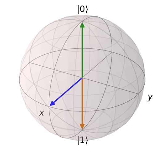
Using global phase invariance to rewrite this as a Bloch vector on the Bloch sphere allows for a useful visualisation:

$$\ket{\psi}=\cos{\frac{\theta}{2}}\ket{0}+e^{\imath\phi}\sin{\frac{\theta}{2}}\ket{1}$$

Where $\theta,\phi$ are the polar and azimuthal angles on this sphere. For example, Figure 1 shows three possible states:

A well-designed algorithm can leverage superposition to perform calculations faster than a classical computer. Maintaining the superposition is therefore vital. However, it is fragile, and can be destroyed by environmental interactions or the decoherence the qubit itself. Another potential source of errors is from miscalibrated gates, which refers to manipulating the state of a qubit imperfectly. This will be discussed in the next section

2.2 Quantum Gates

A quantum gate is a unitary operation which can be applied to one or more qubits ⁶⁷. For this report, I will only discuss single qubit gates. Unitary operations can be visualised as rotating the Bloch vector around some axis by some angle. Thus, gates are usually labelled by the axis-angle pair. For example, an $X180$ gate is a rotation of $\pi$ radians around the $x$ axis. As this flips a $\ket{0}$ to a $\ket{1}$, this is also known as the quantum $\text{NOT}$ gate. A list of commonly-used gates is provided by ⁷⁸.

A gate can be represented by a unitary matrix $U$, which acts by simple matrix multiplication $\ket{\psi}\to U\ket{\psi}$ where $\ket{\psi}=(\alpha,\beta)^T$.

$$\begin{equation}U(\theta,\phi,\lambda)=\begin{pmatrix}\cos{(\theta/2)}&-e^{-\imath\lambda}\sin{(\theta/2)}\\e^{\imath\phi}\sin{(\theta/2)}&e^{\imath(\phi+\lambda)}\cos{(\theta/2)}\end{pmatrix}\end{equation}$$

The general gate matrix is given by Equation 1 ⁹. This means that one can also label a gate with its tuple of angles. For example, the $X180$ gate is given by the tuple $(\pi, 0, 0)$.

The way gates are applied to qubits depends on the physical implementation of the qubit. For the transmon used in this project, gates are enacted by shaped RF pulses. This will be discussed in Section 2.5.

When a gate is applied, there may be a small error in the physical implementation (e.g. noise in the pulse amplitude), causing an incorrect rotation on the Bloch sphere. If all gates have such errors, the errors will compound, rendering the final result unusable. Thus it is important to calibrate gates correctly to minimise such errors. This calibration is known as ‘tuning up’.

One might expect that each gate would have to be tuned up individually. This would take far too long and would be physically impracticable for some systems. Instead, gate decompositions are used. This refers to representing each gate as a combination of some smaller subset of gates, known as the basis, which is chosen so that the basis set spans the space of all possible gates. Then, only the basis gates need to be tuned up. This comes at the cost of implementing multiple physical gates per logical gate, increasing the circuit duration and potential error.

The basis used in this project is the $\text{vZX}$ basis, which includes a single $X90$ gate, and the set of all $Z$ gates. This basis is chosen because Z gates can be implemented in software, instead of hardware, meaning that the only physical gate being implemented is the $X90$ gate. The precise implementation of a $Z$ gate is discussed in Section 2.5. For now, it suffices to say that because they are software gates, they are perfect and error-free, and so no additional error is introduced. The decomposition of a general gate into this basis is given by Equation 2.

$$\begin{equation} U(\theta,\phi,\lambda)=Z(\phi-\pi/2)\cdot X(\pi/2)\cdot Z(\pi-\theta)\cdot X(\pi/2)\cdot Z(\lambda-\pi/2) \end{equation}$$

2.3 Randomised Benchmarking

Randomised benchmarking (RB) is a commonly-used method for calculating the error in a quantum computer ¹⁰. It involves running a series of circuits of increasing length $m$, and measuring the fidelity $f$ between the final and target states. Then, an exponential $f = ar^m+b$ is fitted to the data. The error per gate (EPG) is $1 − r$.

Each circuit is made of a random selection of Clifford gates $C_1C_2\dots C_m$, followed by a final gate $C_{m+1} = (C_1C_2 \dots C_m)^{-1}$ which returns the qubit to $\ket{0}$. Clifford gates are a certain subset of all gates chosen for RB because the result with Clifford gates is the same as the result from randomly sampling from all possible gates ¹⁰. There are $24$ single-qubit Clifford gates, which come pre-defined in QuTiP. For more details, see ⁷¹¹¹².

2.4 Collapse Operators

The gates discussed above are all unitary, meaning they are reversible. However, quantum systems also undergo irreversible processes, the most important of which is decoherence. This means non-unitary operators must also be included in the simulation. Such operators are known as collapse operators ⁸¹³, and depend on the specific process being simulated.

There are two main types of decoherence. The first type is decay, when a qubit relaxes from an excited state back down to the ground. The second is dephasing, when a superposition is lost, and the state becomes an energy eigenstate. The respective collapse operators are

$$C_1=\frac{1}{\sqrt{t_1}}\hat{a},\quad C_2=\frac{1}{\sqrt{t_2}}\hat{a}^\dag\hat{a}$$

Where $\hat{a}$ is the annihilation operator for the system, and $t_1,t_2$ are the characteristic de cay and dephasing times, respectively. The typical values are $\sim 100\thinspace\mu\text{s}$.

2.5 Transmon Physics

There are a large number of possible implementations of a qubit, including trapped ions or atoms, and NMR with organic molecules ¹⁴. The implementation chosen for this project is a type of superconducting circuit known as a transmon ¹⁵. These are widely used in research due to their long coherence times and flexibility. For the purposes of this report, I will ignore the engineering details and focus on their quantum mechanical properties. More rigorous and detailed descriptions are available here ⁶⁷¹⁶.

A transmon can be seen as an anharmonic quantum oscillator. This is the usual quantum harmonic oscillator with a ladder of energy levels, but whose successive energy gaps differ from each other by a constant anharmonicity $\alpha$ (e.g. $\omega_{23}=\omega_{01}+2\alpha$). A typical value is $\omega_{01}/2\pi\approx 5\text{ GHz}$, $\alpha/2\pi\approx -100\text{ MHz}$. The Hamiltonian of a transmon is given by Equation 3 ⁷, where $E_C, E_J$ are parameters of the transmon, and $\hat{a},\hat{a}^\dag$ are the annihilation and creation operators, respectively. I take the ground state and the first excited state to be the logical $\ket{0},\ket{1}$.

$$\begin{equation} \frac{H_0}{\hbar}=-\sqrt{\frac{E_CE_J}{2}}\left(\hat{a}^\dag-\hat{a}\right)^2-E_J\cos{\left[\left(\frac{2E_C}{E_J}\right)^{1/4}\left(\hat{a}^\dag+\hat{a}\right)\right]} \end{equation}$$

Time evolution under this Hamiltonian is predicted by Schrödinger’s equation to add a different time-varying phase to $\ket{0}$ and $\ket{1}$, corresponding to a constant rotation around the $z$ axis on the Bloch sphere. The angular velocity of this rotation is simply the transition frequency $\omega_{01}$. This rotation complicates the simulation of the transmon, and so I transform to a co-rotating frame to eliminate it. To find $\omega_{01}$, one could perform the rotating wave approximation, but this sacrifices accuracy. As there is no analytical way to extract $\omega_{01}$ and $\alpha$ from the full Hamiltonian, I instead use QuTiP to diagonalise the Hamiltonian and extract the eigenenergies:

$$\begin{aligned} \hbar\omega_{01}&=E_1-E_0\\ \hbar\alpha&=(E_2-E_1)-(E_1-E_0) \end{aligned}$$

The transmon can be coupled to an EM field via a driving Hamiltonian given by

$$H_1(t)/\hbar=A(t)\cos{(\omega t+\phi)}\left(\hat{a}^\dag+\hat{a}\right)$$

Where $A(t)$ is some envelope function, $\omega$ is the pulse frequency which determines which transition is excited (and is set to $\omega_{01}$), and $\phi$ is the pulse phase which determines which axis in the $xy$ plane is rotated around on the Bloch sphere (conventionally set so $\phi=0$ is a rotation around the $x$ axis). For the envelope function, I chose a Blackman function, described in Equation 4, where $A$ is the amplitude, $\Gamma$ is the width of the pulse from zero to zero, $\tau$ is the total duration of the gate and $p$ is the padding before and after the pulse. The padding is included because when pulses are physically shaped, there may be ringing or other effects, and the padding ensures that the pulse is not truncated too early. I chose this over a Gaussian because of its smoother and quicker decrease to zero, eliminating discontinuities.

$$\begin{equation} A(t)=\begin{cases} \frac{50\pi A}{42\Gamma}\left(0.42-0.5\cos{\left[\frac{2\pi(x-p-\Gamma)}{\Gamma}\right]}+0.08\cos{\left[\frac{4\pi(x-p-\Gamma)}{\Gamma}\right]}\right)&\text{ if }p<t<\tau-p\\ 0&\text{ otherwise} \end{cases} \end{equation}$$

The utility of the chosen $\text{vZX}$ basis is then clear: to tune up an $X$ gate, only the envelope function $A(t)$ needs to be optimised, while the virtual $Z$ gates are applied by adding a constant phase to all subsequent pulses. For example, $Z(\theta)\equiv \phi\to\phi+\theta$.

One drawback of the transmon implementation is that it has more than two energy levels, and so there is a possibility that the state will ‘leak’ out of the computational subspace and into higher levels. This leakage is caused by the pulse having a finite duration and thus a finite bandwidth which may extend to the next transition frequency. It can be reduced via DRAG shaping ¹⁷. The pulse function $A(t)\cos{(\omega t)}$ is generalised to

$$I(t)\cos{[(\omega+\delta)t+\phi]}+Q(t)\sin{[(\omega+\delta)t+\phi]}$$

Where $I, Q$ are the ‘in-phase’ and ‘quadrature’ components of the envelope. This reduces to the original pulse when $I(t) = A(t)$ and $Q(t) = 0$. DRAG shaping is instead when $Q(t)=\lambda T(t)/\alpha$, where $\lambda$ is known as the DRAG parameter. This suppresses leakage by reducing the frequency component of the pulse near the $\omega_{12}$ transition. This however also causes a small AC-Stark effect, which makes the Bloch vector precess around the $z$ axis. This precession can be controlled by detuning the pulse appropriately via $\delta$. Thus, the only pulse parameters which must be optimised are $A,\lambda,\delta$.

2.6 Superoperators

Consider a single quantum system with $n$ states, such as a transmon. A general pure state of the system is represented as a vector $\ket{\psi}$ in a Hilbert space of dimension $n$, whose basis is conventionally chosen to be the energy eigenstates $\ket{n}$. An operation on this state is known as a quantum channel $\ket{\psi}\to\Lambda(\ket{\psi})$. A unitary channel such as a gate is represented as an $n\times n$ unitary matrix mapping the Hilbert space to itself. However, the result of a non-unitary channel such as decoherence or a pulse cannot be written as a pure state, but as a density matrix $\rho$.

To apply a quantum channel to a mixed state, we must shift to the superoperator formalism, by transforming to a Hilbert space $H_n\otimes H_n$. The basis for the new space is any spanning set of $n\times n$ Hermitian matrices $\mathcal{B}={B_1,B_2,\dots,B_{n^2}}$. For this project, I chose the basis to be the generalised Gell-Mann matrices ¹⁸, which reduce to the Pauli matrices for $n = 2$.

The general state of the system is now written as the ‘superket’ $\ket{\rho}\rangle$, whose components are $\ket{\rho}\rangle_i=\braket{\braket{i|\rho}}=\text{Tr }B_i\rho$. For example, the density matrix identical to the first element of the basis $\rho=B_1$ would become $\ket{\rho}\rangle=(1,0,0,\dots,0)^T$ in the new Hilbert space.

The quantum channel $\Lambda$ can then be written as a Pauli Transfer Matrix $R_\Lambda$, which maps superkets. It is an $n^2\times n^2$ matrix whose elements are given by ¹³¹⁹

$$(R_\Lambda)_{ij}=\braket{\braket{B_i|\Lambda(B_j)}}=\text{Tr }[B_i\Lambda(B_j)]$$

Thus, the PTM for a particular channel is found by applying the channel to the set of basis states, and taking the inner product of the transformed basis states with the original basis states. This definition generalises to both a complicated channel such as a pulse, and a simple ideal channel such as a unitary gate.

The PTM is useful because it acts multiplicatively, even for non-unitary maps: $\ket{\Lambda(\rho)}\rangle=R_\Lambda\ket{\rho}\rangle$. Thus the effect of a series of channels is given by

$$\ket{\Lambda_2\circ\Lambda_1(\rho)}\rangle=R_{\Lambda_2}R_{\Lambda_1}\ket{\rho}\rangle$$

Then, as I have chosen to use the vZX decomposition, the PTM for a given gate can be found by multiplying together the $X90$ PTM and the ideal vZ PTMs as described by Equation 2. Only one pulse needs to be tuned up to be able to use PTMs for simulation.

As matrix multiplication is much quicker than simulating time evolution, the superoperator formalism can be used to perform simulations much faster while retaining the same degree of accuracy.

Finally, by converting the PTM to a ‘process’ or $\chi$ matrix and comparing to the ideal matrix, it is possible to deduce the errors present, and potentially their sources ²⁰. Interconversions between different types of superoperator matrix are detailed in ¹³ but this was not implemented and is a promising area for future work.

2.7 QuTiP

QuTiP ⁸ is a Python library commonly used for quantum simulations. It has several useful features including proper handling of states and operators, easy Bloch sphere visualisation, circuit-level and pulse-level simulation, and an inbuilt list of single-qubit Clifford gates.

Pulse-level simulation is performed by the master equation ²¹ solver mesolve, which takes a Hamiltonian, initial state, and list of collapse operators, and propagates the state forward in time. The pulse is effected via a time dependent Hamiltonian. However, dynamically changing the Hamiltonian is not possible, and so multiple layers of wrapper functions were required when shifting pulse phases.

The eigenenergy method of finding the frequency and anharmonicity of a transmon from Section 2.5 was implemented in QuTiP by recursively forming a Hamiltonian, finding its eigenenergies, and then using scipy’s ‘optimize’ module to converge on the desired values. This could not be avoided as the Hamiltonian had to be passed to ‘mesolve’, but as it was a one-time operation it was not a significant issue

It was not possible to dynamically implement the rotating frame transformation in QuTiP, and instead the transformation was applied at the end of the simulation without loss of accuracy by rotating each simulated state by some calculated amount. Finally, the superoperator formalism is not yet implemented properly in QuTiP version 4.7.1, and so custom code was developed to form the PTM and convert to Choi and $\chi$ matrices.

3 Simulations and Results

3.1 Tuning up a single gate

For this project, I chose my transmon to have $\omega_{01}/2\pi=3981\text{ MHz}$ and $\alpha/2\pi = -199\text{ MHz}$. I also chose gates to be $50\text{ ns}$ long, with a padding of $2\text{ ns}$ before and after the pulse.

Using QuTiP’s framework, I set up a transmon class with a user-defined number of levels $n$, Hamiltonian $H_0$, and decay and dephasing times $t_1,t_2$, which were initially set to be infinite. Then, the pulse was included by adding the DRAG-corrected driving Hamiltonian and defining the pulse parameters.

Given I was using the $vZX$ decomposition, I only had to tune up the $X90$ gate by optimising $A,\delta,\lambda$. The first two had to be optimised for fidelity between the final state and the target state, and the latter had to be optimised to minimise leakage out of the computational subspace of $\ket{0},\ket{1}$.

To perform this optimisation, I varied each parameter in turn, and plotted fidelity or 1-leakage as a function of the parameter. The optimal values were then found by fitting the curve with a spline function and finding the maximum. This was repeated multiple times to find a global maximum. An example of the curve found from optimising amplitude is given in Figure 2.

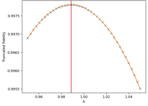
The optimal pulse parameters were $A=0.97837\text{ V m}^{-1}, \delta/2\pi=7.78273\text{ Hz}$, and $\lambda=1.00293$. The gate error was $1.1\times 10^{-4}$. Of this, $1\times 10^{-4}$ was leakage, leaving approximately $10^{−5}$ from miscalibration. This is a very good result, and shows that the pulse is almost ideal.

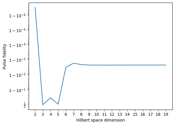
The question of how many levels to use in the simulation was also investigated. Using the non-optimised parameters $A=1,\lambda=\delta=0$, I varied the number of levels in the transmon and got the data in Figure 3. The fidelity for $n = 2$ is so high because $A = 1$ is the theoretically optimal value. The reason for the sharp dips for $n = 3, 4, 5$ is unknown and warrants further research. The fidelity appears to become stable at $n = 10$, which was the value I used for this project.

3.2 Spectroscopy

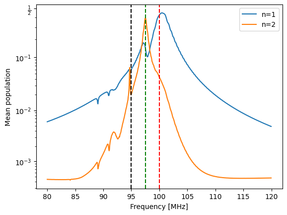
To check that the simulation was correctly implementing multi-photon transitions (which are required for the $n=0\to 2$ transition, which is electric dipole forbidden), I performed a spectroscopy experiment with a dummy transmon $n=10, \omega_{01}/2\pi=100\text{ Hz}, \alpha/2\pi=-5\text{ Hz}$ by applying a continuous sine wave with variable frequency and plotting the level populations. The result is shown in Figure 4. The red and black dashed lines are the expected peaks at $\omega_{01}$ and $\omega_{12}$ respectively. There is also a peak at $\omega_{02}/2$ (green dashed), which corresponds to a two-photon transition. This means that multi-photon transitions are being correctly simulated.

3.3 Collapse operators and noise

I then chose the decay and dephasing times for the qubit to be $t_1=10\thinspace\mu\text{s}$ and $t_2=20\thinspace\mu\text{s}$. The theoretical decoherence error for one pulse was $1.66\times 10^{-3}$, using the equation in ²². After decoherence effects were added, the error of a single pulse was $2.00\times 10^{-3}$, with $0.28\times 10^{-3}$ leakage. The error unaccounted for was $6\times 10^{-5}$. This demonstrates that the pulse fidelity was coherence-limited.

I then investigated the effects of noise in the pulse amplitude and phase. I simulated the pulse with a phase and amplitude drawn from a normal distribution of varying width, and plotted the results, shown in Figure 5. Note that here, the state was truncated to the computational subspace before fidelity was measured. These data allow a user to estimate what the maximum amount of noise in their control system can be to still achieve a certain threshold fidelity, although it would have to be confirmed by an experiment on a real device.

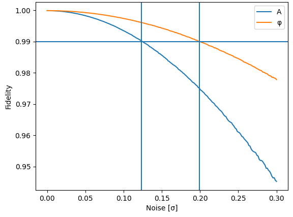
The fidelity curves would be identical under rescaling because $A$ affects the final polar angle on the Bloch sphere, while $\phi$ affects the azimuthal angle. Thus, the variation in fidelity with noise is expected to be similar due to spherical symmetry.

3.4 Circuit simulation

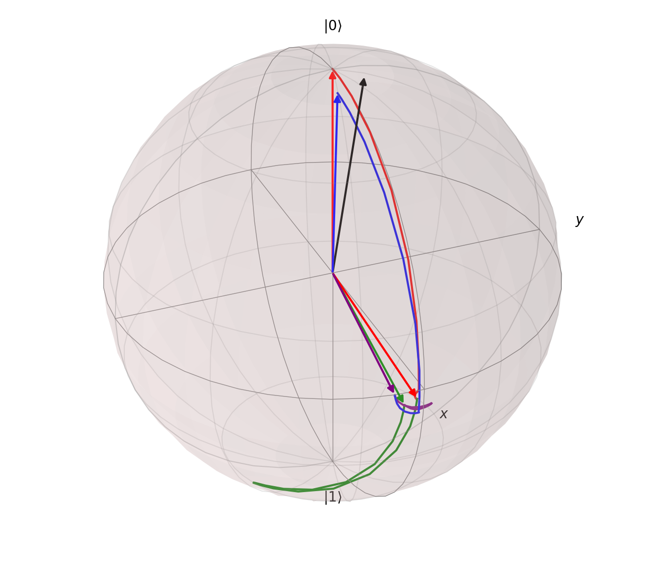
I then implemented the next layer of abstraction, which was to specify a circuit and have each gate automatically broken down into a set of pulses with the $vZ$ gates applied by shifting the phase of each pulse as required. An example of the evolution under the circuit $X90-Z90-Z180-Y90$ is shown in Figure 6, where the lines denote the path taken between states. The arrows correspond to the state of the qubit after each logical gate (which corresponds to two physical gates). The final state (black) had a fidelity of $0.98583$, which agrees well with the expected value, taking into account gate error and decoherence.

3.5 Implementing the superoperator formalism

I then moved on to implementing the superoperator formalism. Having tuned up the $X90$ gate, I created its PTM as described in Section 2.6. I applied both to $1000$ random initial states and found the average fidelity between the pulse and PTM results to be $1-3\times 10^{-7}$, meaning perfect agreement. Having confirmed this, I made a function to return the ideal PTM for a $Z\theta$ gate, where $\theta$ is the angle of rotation. This was done by transforming the Gell-Mann matrices with$\Lambda(B_i)=ZB_iZ$ where $Z$ is the $z$ rotation matrix. Using this, I implemented the same circuit simulation capabilities with PTMs as with pulses.

3.6 Randomised benchmarking

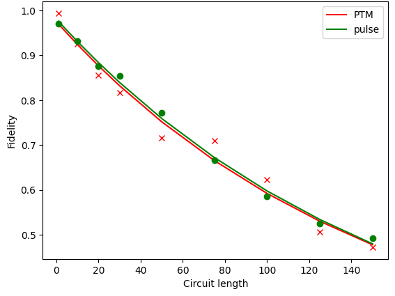
I then performed RB using both pulse simulation and the PTM method. I simulated circuits of increasing length up to $m = 150$, $30$ times each, and plotted fidelity against length in both cases to get the plot in Figure 7. The fitted curves agree very well, and the EPGs are $3.67\times 10^{-3}$ and $3.63\times 10^{-3}$ respectively. The expected EPG is $3.54\times 10^{-3}$, demonstrating a good agreement. The reason for the discrepancy warrants further research, and could be due to a number of factors including imperfect DRAG correction or too-coarse timesteps. However, the PTM simulation was much quicker. Exact RB duration was not measured due to implementation constraints, but in a dummy run, pulse simulation took $16\text{ min}$ to simulate a circuit with $101$ logical gates, while PTM simulation took $2\text{ min}$. Upon analysis, the bottleneck was creating the $vZ$ gate PTMs, and so optimising this function could provide further speed boosts.

Nevertheless, this result demonstrates that the superoperator formalism is accurate and efficient, and potentially a powerful simula tion tool. An example of a procedure a research group could follow to exploit this is as follows: first, set up the physical qubit and tune up the $X90$ gate. Then, apply this gate to all of the states corresponding to the superoperator basis. Record the results, and create a PTM. Then, simulate and physically perform RB, and compare the results. If they match, then a perfect representation of the physical qubit has been found. This can then be used to simulate any circuit, and test the effects of modifying any parameters, such as of the qubit. For example, the decoherence times could be set to infinity, allowing prediction of exactly how much improving the qubit coherence would affect the error rate.

To simulate the addition of noise, the PTM would have to be modified, and further work is required to determine the precise change. Indeed, superoperators provide a powerful way of doing this: by modulating the noise in the driving pulse and forming a PTM each time, the correspondence can be established and the original examined to determine sources of noise.

4 Conclusions

The aim of this project was to show that it is possible to simulate the time evolution of a single transmon qubit using the superoperator formalism much faster than existing numerical methods such as solving the master equation. I achieved this result, speeding up simulations by an order of magnitude while retaining accuracy, as shown by the agreement between both single-pulse results and RB results.

This speed-up is significant, and could be used to simulate a large number of circuits in a short time. This could be used to identify the sources of error in a system, or to optimise the parameters of a circuit.

However, the EPGs returned by RB did not agree exactly, and so it would be necessary to confirm whether this was due to simulation issues such as the time steps being too large, or the randomness of decoherence being improperly modelled.

Furthermore, this project dealt with only a single qubit with n = 10 levels. Simulations of multi-qubit systems would involve modelling cross-talk and other effects, and it remains to be seen whether this method is possible and practical for such a situation.

The protocol outlined at the end of the last section outlined an empirical way to establish the relationship between pulse noise and the PTM. This could be extended analytically if the error decomposition from ²⁰ were implemented. This would allow the user to directly identify the sources and types of error in their system, and work to reduce them, rather than identifying them indirectly.

The PTM method could be further sped up in a number of ways. One would be to optimise the function creating the vZ PTMs, as this was the main bottleneck. Another way would be via a technique known as effective Hamiltonians ²³²⁴. These work on the principle that the evolution of a simulated system need only match that of a real system at the measurement times; what happens in between is irrelevant. This means that the evolution of the system can be simulated using a much simpler Hamiltonian, which matches the real Hamiltonian at the measurement times, but which is much faster to compute. This would allow a significant speed boost, but testing would determine whether it would need to be used in combination with the PTM approach, or whether it would be fast enough on its own.

Additional next steps for this project would be to validate these results on an actual device. Checking that the pulse simulation matches real results is vital to ensure the PTM simulation is a useful tool in real research. Whether or not the results of this project are useful in practice will depend on this, but nevertheless, they represent a potentially useful proof-of-concept off of which further work can be done.

References